1 Day 1: Math Prerequisites
Sources for this page: d2l.ai, Dive into Deep Learning, Preliminaries (§2.3 Linear Algebra, §2.5 Calculus, §2.6 Probability and Statistics) — CC BY-SA 4.0; Wikipedia, Dot product, Gradient, Chain rule, Bayes’ theorem — CC BY-SA 4.0. Text below is written from scratch, not copied, following these ideas; standard results (the geometric dot-product formula, the chain rule, Bayes’ theorem) are stated in the conventional way found in any of these sources.
This is a refresher, not a first encounter. The goal isn’t to re-teach linear algebra, calculus, or probability from zero — it’s to consolidate exactly the pieces this course actually uses, work through them with real numbers, and show you where each one shows up later, so none of it feels like disconnected math-for-its-own-sake. There’s no coding today; that’s Day 2 — though the notebook linked at the bottom lets you check today’s by-hand answers in code if you’re curious.
1.1 Learning goals
By the end of this session you should be able to compute a dot product by hand and interpret it geometrically, take a partial derivative of a simple multivariable function and use it to run a step of gradient descent, and apply Bayes’ rule to a concrete conditional-probability problem.
1.2 Vectors, matrices, and the dot product
A vector is just an ordered list of numbers, and a matrix is a rectangular grid of them. You already know how to add two vectors (add corresponding entries) and how to scale one (multiply every entry by the same number). The one operation worth slowing down on is the dot product:
\[ \mathbf{w} \cdot \mathbf{x} = w_1 x_1 + w_2 x_2 + \dots + w_n x_n \]
This is nothing more than “multiply corresponding entries, then add everything up” — but it’s worth naming because it shows up constantly. It’s a weighted sum: each \(x_i\) contributes to the total in proportion to its own weight \(w_i\).
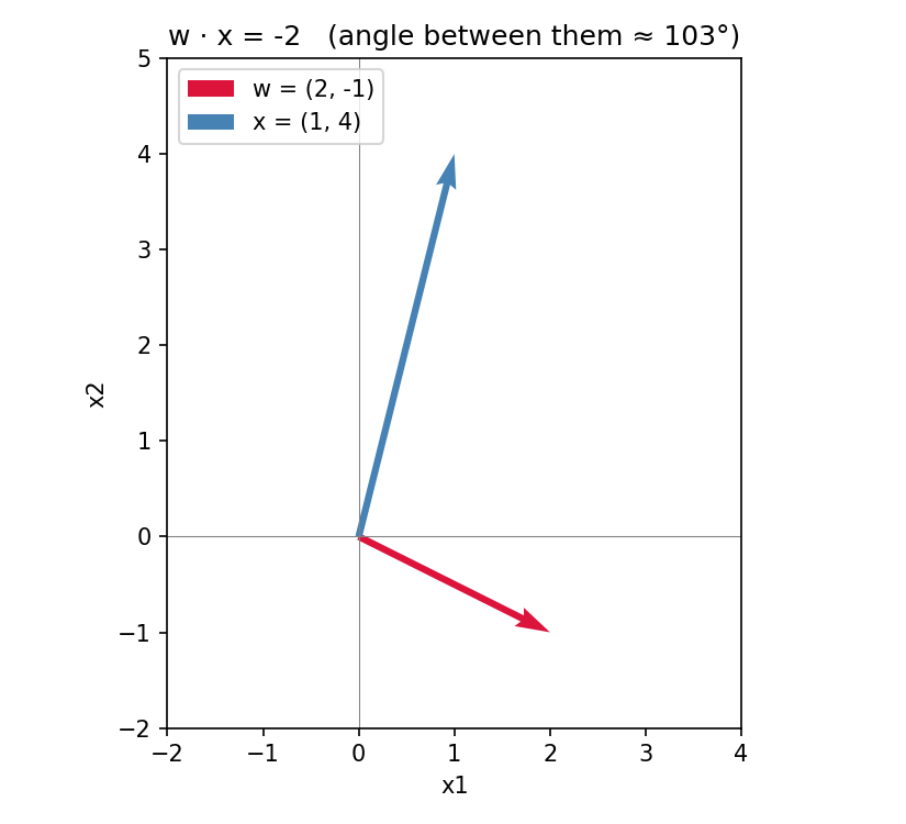
Worked example. For \(\mathbf{w} = (2, -1)\) and \(\mathbf{x} = (1, 4)\):
\[ \mathbf{w} \cdot \mathbf{x} = (2)(1) + (-1)(4) = 2 - 4 = -2 \]
The dot product also has a geometric meaning that’s worth having in your head, not just the arithmetic definition:
\[ \mathbf{w} \cdot \mathbf{x} = \lVert \mathbf{w} \rVert \, \lVert \mathbf{x} \rVert \cos\theta \]
where \(\theta\) is the angle between the two vectors and \(\lVert \cdot \rVert\) denotes a vector’s length. This tells you the sign of a dot product for free, without computing anything: it’s positive when the angle between the vectors is less than 90° (they point in broadly the same direction), zero when they’re exactly perpendicular, and negative when the angle exceeds 90° (they point in broadly opposite directions). In the worked example above, \(\mathbf{w}\) and \(\mathbf{x}\) are about 103° apart — just past perpendicular — which is exactly why their dot product came out negative:
Why does this one specific computation deserve a whole session’s worth of attention before we’ve even started the course proper? Because it reappears, unchanged, in two very different-looking places later in this course. A profile score (Day 6) — the standard way of asking “how well does this sequence match a known family?” — is computed by multiplying each position’s observed value by a position-specific weight and summing. And a perceptron (Day 7), the simplest kind of artificial neuron, computes its output the exact same way: a dot product between a weight vector and an input vector. When we get there, you’ll already know the arithmetic and the geometric intuition; the only new part will be what to do with the result.
Matrix–vector and matrix–matrix multiplication are the same idea done many times at once: a matrix–vector product is just a batch of dot products, one per row of the matrix. For example,
\[ \begin{pmatrix} 2 & -1 \\ 0 & 3 \end{pmatrix} \begin{pmatrix} 1 \\ 4 \end{pmatrix} = \begin{pmatrix} (2)(1) + (-1)(4) \\ (0)(1) + (3)(4) \end{pmatrix} = \begin{pmatrix} -2 \\ 12 \end{pmatrix} \]
— the first entry of the result is exactly the dot product worked out above; the second is a new dot product between the matrix’s second row and the same vector \(\mathbf{x}\).
1.3 Derivatives and the gradient
A derivative tells you how much a function’s output changes for a small change in its input — the slope of the tangent line at a point. If you’ve seen this before, that’s the whole idea; what’s worth reviewing is what happens once there’s more than one input.
A partial derivative of a function of several variables, written \(\partial y / \partial x_i\), is computed by treating every variable except \(x_i\) as a constant and differentiating as usual. If you stack all of a function’s partial derivatives into a single vector, you get its gradient:
\[ \nabla y = \left( \frac{\partial y}{\partial x_1}, \dots, \frac{\partial y}{\partial x_n} \right) \]
Worked example. For \(f(x_1, x_2) = 3x_1^2 + 2x_1 x_2\):
\[ \frac{\partial f}{\partial x_1} = 6x_1 + 2x_2, \qquad \frac{\partial f}{\partial x_2} = 2x_1 \]
(For \(\partial f/\partial x_1\), \(x_2\) is held constant, so \(2x_1 x_2\) differentiates like \(2x_2 \cdot x_1\), giving \(2x_2\); for \(\partial f/\partial x_2\), \(x_1\) is held constant, so \(3x_1^2\) contributes nothing and \(2x_1 x_2\) differentiates to \(2x_1\).) At the point \((1, 2)\):
\[ \nabla f(1, 2) = (6(1) + 2(2), \ 2(1)) = (10, 2) \]
Geometrically, the gradient at a point tells you two things at once: the direction in which the function increases fastest, and (via its length) how steeply. Point yourself in the opposite direction, and you’re headed downhill as fast as possible from where you’re standing.
That last sentence is the entire idea behind gradient descent, which Day 7 uses to train the perceptron introduced above. Given a function that measures how wrong a model’s predictions are (a loss function), repeatedly step a small amount in the direction opposite its gradient, and the error goes down. Concretely, the update rule is
\[ x_{n+1} = x_n - \eta \, f'(x_n) \]
where \(\eta\) (eta) is a small positive learning rate controlling the step size. Let’s watch this actually converge, one step at a time, for the one-variable function \(f(x) = (x - 3)^2\), whose derivative is \(f'(x) = 2(x-3)\), starting from \(x_0 = 0\) with \(\eta = 0.3\):
| \(n\) | \(x_n\) | \(f(x_n)\) | \(f'(x_n)\) | \(x_{n+1} = x_n - 0.3 f'(x_n)\) |
|---|---|---|---|---|
| 0 | 0.000 | 9.00 | -6.00 | 1.800 |
| 1 | 1.800 | 1.44 | -2.40 | 2.520 |
| 2 | 2.520 | 0.23 | -0.96 | 2.808 |
| 3 | 2.808 | 0.037 | -0.384 | 2.923 |
Notice two things: \(x_n\) is closing in on 3 (the true minimum, where \(f'(x) = 0\)), and the steps themselves shrink as it gets closer, purely because the derivative shrinks — nobody had to manually decrease \(\eta\). This exact table-of-iterations idea is what you’ll watch happen inside a real model’s training loop, starting Day 7, except with many weights being updated at once via the gradient vector instead of one number via a single derivative.
One more idea from calculus matters more than any other for this course: the chain rule. For a composite function \(y = f(g(x))\), its derivative is
\[ \frac{dy}{dx} = \frac{df}{dg} \cdot \frac{dg}{dx} \]
— the derivative of a function of a function is the product of their individual derivatives. It looks unremarkable written down, but it is, quite literally, the one idea backpropagation (Day 10) is built from: a neural network’s output is a function of a function of a function of its weights, and the chain rule is what lets us compute how each weight, however deeply buried, should change, by multiplying together the derivatives of every function it passes through on the way to the output.
1.4 Probability basics
A random variable takes on different values with different probabilities — a discrete one (like a die roll) has a countable list of outcomes, each with a probability; a continuous one (like a measured concentration) has a probability density instead. The expectation of a random variable is its probability-weighted average value:
\[ \mathbb{E}[X] = \sum_i x_i \, P(X = x_i) \]
Worked example. For a fair six-sided die, each outcome has probability \(1/6\), so
\[ \mathbb{E}[X] = \frac{1+2+3+4+5+6}{6} = 3.5 \]
Note that 3.5 isn’t even a possible outcome of a single roll — expectation is a long-run average, not a prediction of any one result.
Conditional probability — the probability of one event given that another has occurred, written \(P(A \mid B)\) — and Bayes’ rule, which lets you flip a conditional probability around, are worth having solid before Day 6, where they’re exactly the machinery underneath a Hidden Markov Model. Bayes’ rule follows directly from the definition of conditional probability (\(P(A \mid B) = P(A \cap B)/P(B)\), applied both ways round) and reads:
\[ P(A \mid B) = \frac{P(B \mid A) \, P(A)}{P(B)} \]
Worked example (the classic illustration of why this matters): a diagnostic test for a rare condition affecting 1% of a population is 95% accurate on people who have it (\(P(\text{positive} \mid \text{disease}) = 0.95\)) and gives a false positive 5% of the time on people who don’t (\(P(\text{positive} \mid \text{no disease}) = 0.05\)). If someone tests positive, what’s the actual probability they have the condition?
\[ P(\text{disease} \mid \text{positive}) = \frac{P(\text{positive} \mid \text{disease}) \, P(\text{disease})}{P(\text{positive})} \]
The denominator, \(P(\text{positive})\), has to account for positives from both groups: \(P(\text{positive}) = (0.95)(0.01) + (0.05)(0.99) = 0.0095 + 0.0495 = 0.059\). So
\[ P(\text{disease} \mid \text{positive}) = \frac{(0.95)(0.01)}{0.059} \approx 0.161 \]
Despite a 95%-accurate test, a positive result only means about a 16% chance of actually having the condition — because the condition is rare, false positives from the large healthy population outnumber true positives from the small affected one. This kind of reasoning — combining a prior probability with new evidence — underpins the loss functions used everywhere from Day 7 onward: minimizing a loss function during training is, in most of the models in this course, equivalent to finding the model parameters that make the observed data most probable.
1.5 Practice problems
Work through these by hand first, then check your answers.
- Compute \((2, -1, 3) \cdot (1, 4, 0)\).
- For \(f(x_0, x_1) = 3x_0^2 + 2x_0 x_1\), compute \(\nabla f\) at the point \((1, 2)\).
- A fair six-sided die is rolled once. What is \(P(\text{even} \mid X > 3)\) — the probability of an even result, given that the result exceeds 3?
- \((2)(1) + (-1)(4) + (3)(0) = 2 - 4 + 0 = -2\).
- \(\partial f/\partial x_0 = 6x_0 + 2x_1 = 6(1) + 2(2) = 10\); \(\partial f/\partial x_1 = 2x_0 = 2(1) = 2\). So \(\nabla f(1,2) = (10, 2)\).
- \(X > 3\) means the outcome is 4, 5, or 6 — three equally likely outcomes. Of those, 4 and 6 are even: two out of three. So \(P(\text{even} \mid X > 3) = 2/3\).
1.6 The notebook
notebooks/day01-math-in-code.ipynb recomputes every worked example and practice problem above in code — the dot product, the gradient (checked two ways: by hand and via automatic differentiation), and the die-roll probabilities (checked two ways: exactly, and by simulating a few hundred thousand rolls) — so you can confirm code and math agree before Day 2 introduces the code side properly. The version below is a static, read-only copy; open it in Google Colab via the badge at the top of the notebook page to edit and run it yourself.
1.7 What’s next
Day 2 takes every idea above and writes it in code the idiomatic way: the dot product becomes a line of PyTorch, and the gradient becomes something the framework computes for you automatically.