3 Day 4: Sequence Alignment
Sources for this page: Petras Kundrotas’s KB8029 lecture “Sequence Alignment” (Feb 2026) — this page follows its structure and worked examples, adapted and shortened for this book, not copied verbatim; the two figures below (orthologs/paralogs; the completed Needleman-Wunsch traceback) are taken directly from that lecture’s slides; Dayhoff, Schwartz & Orcutt (1978), Atlas of Protein Sequence and Structure, pp. 345-352 (origin of the PAM matrices); Henikoff & Henikoff (1992), PNAS 89:10915-10919 (origin of the BLOSUM matrices); Wikipedia, Needleman–Wunsch algorithm, Smith–Waterman algorithm — CC BY-SA 4.0.
3.1 Learning goals
By the end of this session you should be able to explain why sequence alignment needs a dedicated algorithm rather than brute-force comparison, work a small global alignment by hand using dynamic programming, explain the difference between global and local alignment, and explain what distinguishes the PAM and BLOSUM families of substitution matrices.
3.2 Why alignment needs an algorithm
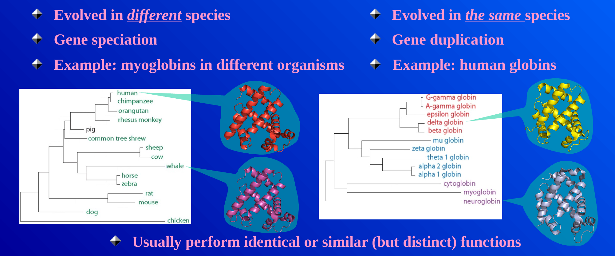
Two sequences are called homologous if they share a common evolutionary origin — a qualitative, yes/no property. Identity and similarity are how homology gets measured in practice: identity is the fraction of positions with the exact same residue; similarity is looser, also counting positions with residues that share physicochemical properties (e.g. two hydrophobic residues). Homologous proteins found in different species are orthologs; homologous proteins found within the same genome (arising from gene duplication) are paralogs. Orthologous myoglobins across mammals, and the family of paralogous human globins (hemoglobin, myoglobin, neuroglobin, and others, all descended from gene duplications), are the standard example:
When two sequences happen to be the same length, measuring identity is trivial — just place one under the other and count matches. Real sequences, though, differ in length because of insertions and deletions over evolutionary time, and where you choose to place one sequence under the other changes the answer dramatically. Two example globin sequences that are 21.5% identical when aligned correctly can look as low as 4% identical if placed naively.
Could you just try every possible placement and keep the best one? For two sequences of length \(n\), allowing gaps, the number of possible alignments grows so fast that for \(n = 100\) it’s already around \(10^{59}\) — utterly infeasible to search exhaustively. This is exactly why dynamic programming algorithms exist for this problem: they find the guaranteed-optimal alignment without ever checking most of the possibilities.
3.3 Dynamic programming: Needleman-Wunsch and Smith-Waterman
The idea: build a matrix \(V\) with one extra row and column (for handling the sequence starts), fill it in using a simple rule, then trace back through it to read off the best alignment. Every cell \(V(i,j)\) is filled as the best of three options — extend a match/mismatch diagonally, or open a gap from above or from the left:
\[ V(i,j) = \max \begin{cases} V(i-1,j-1) + s(x_i, y_j) \\ V(i-1,j) + g \\ V(i,j-1) + g \end{cases} \]
where \(s(x_i, y_j)\) is a substitution score (see below) and \(g\) is a gap penalty. Worked example: align \(x = \texttt{GCAT}\) against \(y = \texttt{GAC}\), with match \(= +1\), mismatch \(= -1\), gap \(= -1\):
| G | A | C | ||
|---|---|---|---|---|
| 0 | -1 | -2 | -3 | |
| G | -1 | 1 | 0 | -1 |
| C | -2 | 0 | 0 | 1 |
| A | -3 | -1 | 1 | 0 |
| T | -4 | -2 | 0 | 0 |
Tracing back from the bottom-right corner (score 0) gives the optimal global alignment:
G C A T
G - A C
— G matches G, C is deleted, A matches A, and T is (mis)matched to C, for a total score of \(1 - 1 + 1 - 1 = 0\).
The same idea, at the scale it’s actually used: two 12-13 residue protein sequences, with the completed matrix and its full traceback path highlighted:
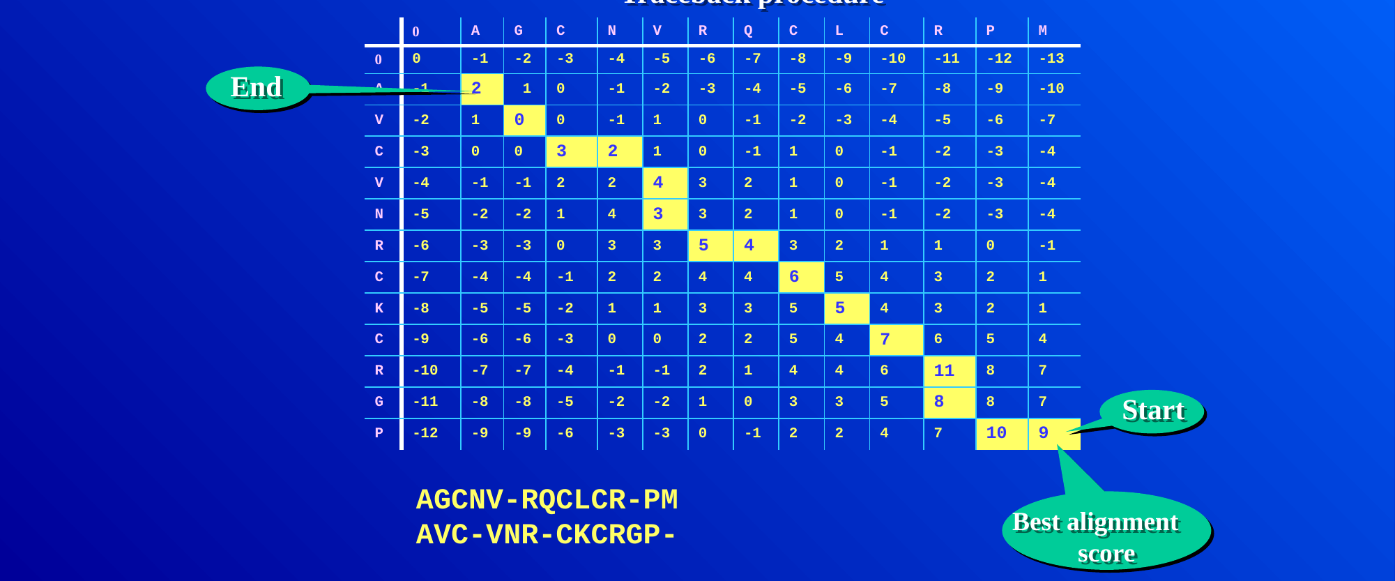
This particular algorithm — Needleman-Wunsch — produces a global alignment: the entire length of both sequences is forced into the result, gaps and all. Smith-Waterman is the same idea adapted for local alignment — finding the best-matching sub-region rather than aligning end-to-end — achieved with one change: negative values in the matrix are reset to zero, and the traceback starts from the highest-scoring cell anywhere in the matrix (not necessarily the bottom-right corner) and stops as soon as it hits a zero.
3.4 Substitution matrices: PAM and BLOSUM
The scores \(s(x_i, y_j)\) above aren’t arbitrary — they come from observing real evolutionary substitutions. Two families dominate:
- PAM (Point Accepted Mutations; Dayhoff, Schwartz & Orcutt, 1978) is based on global alignments of closely related proteins, built from an explicit evolutionary model: sequences are arranged into phylogenetic trees, ancestral sequences are inferred, and substitutions are counted along the tree’s branches. Only PAM1 (calibrated so 99% of residues are unchanged over that evolutionary distance) is derived directly from data — every other PAM matrix is extrapolated from it by repeated matrix multiplication (\(\mathbf{M}^{250}\) for PAM250, etc.).
- BLOSUM (BLOcks SUbstitution Matrix; Henikoff & Henikoff, 1992) is based on local, ungapped alignments of distantly related proteins instead: substitution frequencies are counted directly from conserved blocks of real multiple alignments, with no phylogenetic tree and no extrapolation — each BLOSUM matrix (BLOSUM45, BLOSUM62, BLOSUM80, …) is derived independently from the others.
One easy source of confusion: the two families’ numbering runs in opposite directions. A higher PAM number means a more distant comparison (PAM250 suits more divergent sequences than PAM100); a higher BLOSUM number means a closer comparison (BLOSUM80 suits more similar sequences than BLOSUM45) — the opposite trend.
3.5 Multiple sequence alignment
Extending pairwise alignment to more than two sequences at once has four main strategies:
| Approach | Programs | Speed | Accuracy | Guide-tree dependence | Refinement |
|---|---|---|---|---|---|
| Exact — extend dynamic programming to \(N\) dimensions; only feasible for \(N \le 5\) sequences | — | — | Optimal (for small \(N\)) | None | — |
| Progressive — align the most similar pair first, then progressively add sequences/profiles, guided by a tree built from all pairwise distances | ClustalW | Fast | Moderate | High | No |
| Iterative — start from a progressive alignment, then repeatedly re-score and re-align subsets to improve it | MUSCLE | Medium | High | Moderate | Yes |
| Consistency-based — favor alignments that agree with each other transitively (if A aligns with B and B aligns with C, prefer an alignment where A also aligns with C accordingly) | T-Coffee | Slow | Very high | Low | Yes |
The pattern is a genuine speed/accuracy tradeoff: progressive is fast but an early mistake in the guide tree propagates forward uncorrected; iterative and consistency-based methods spend more computation to correct exactly that weakness.
Building the guide tree for progressive alignment uses exactly the kind of hierarchical clustering you’d use on any distance matrix: treat every sequence as its own cluster, repeatedly merge the closest pair of clusters, and stop once only one cluster remains — the merge order is the order sequences get aligned in.
3.6 The lab
A light, tool-based exercise rather than a full lab (Day 5 gets the full lab, once BLAST is covered too): use EMBL-EBI’s pairwise and multiple alignment tools on real sequences, and confirm that a tool’s reported score and alignment match what the dynamic-programming matrix above would predict for a small case.
3.7 What’s next
Day 5 asks a different question about the same underlying problem: exact dynamic programming like Needleman-Wunsch doesn’t scale to searching a new sequence against an entire database — that’s what BLAST’s heuristic is for. Day 6 goes a step further and asks what to do once you have many aligned sequences rather than two: build a profile.